Introduction
One of the features that greatly intrigued me was the implementation of a visually appealing procedural grass system. This system would enable the dynamic spawning of individual grass blades within a procedurally generated world. However, I aimed to avoid using billboards and instead leverage modern technologies to create a more visually appealing result.
Basic implementation
The most basic implementation consists of using Graphics.DrawMeshInstanced to render the mesh with the desired material in different positions. To achieve this, we create a compute shader, which we’ll refer to as the “distributor shader,” that utilizes a height map to distribute various points representing the new positions of the grass. These points are determined using a variable called density, and with the help of a simple SamplerState, we can obtain specific UV coordinates to gather points on the texture. From there, we calculate the world position concerning the texture and create a grass data object. Later, this compute buffer is assigned to a regular vertex and fragment shader that colors the point and positions it at its corresponding world position. However, several optimizations can be made in this process. The primary challenge lies in the presence of multiple limitations. DrawMeshInstanced has a performance threshold for the number of meshes that can be rendered simultaneously, compute buffers have a size limit before they consume the entire GPU memory, and overall scalability is lower than desirable.

Initial attempt at procedurally spawning grass blades
Optimization 1: Frustum culling
The first step is to apply frustum culling to all the grass, which limits the amount of grass being rendered to only what is visible by the camera. To achieve this, we run a compute shader before drawing the mesh. This shader iterates through all the points and removes those that are not within the camera’s field of view. We utilize the projection matrix and the transformation matrix to exclude points outside the frustum. No visual adjustments are required in this process.
//Frustrum culling
//Grass blade position
float4 position = float4(_GrassData[id.x].position.xyz+float3(_TerrainOffset.x,0,_TerrainOffset.y), 1.0f);
float displacement = _GrassData[id.x].displacement; //Grass blade height
float4 viewspace = mul(MATRIX_VP, position); //Get the viewspace matrix
float3 clipspace = viewspace.xyz; //Save the w value

clipspace /= viewspace.w;

clipspace.x = clipspace.x / 2.0f + 0.5f;
clipspace.y = clipspace.y / 2.0f + 0.5f;
clipspace.z = viewspace.w;
//Scale it accordingly

//Initial quick elimination from frustrum culling
bool inView = clipspace.x < -0.2f || clipspace.x > 1.2f || clipspace.z < -0.1f ? 0 : 1;
float dist = distance(_CameraPosition.xz, position.xz);
bool withinDistance = dist < _Distance; //Distance culling
Optimization 2: Occlusion culling
In some cases, a huge part of the grass could be occluded by external factors, like a house, wall or boxes. We can remove those unnecessary grass blades through a simple occlusion culling algorithm. To implement it we will generate at every buffer (via a command buffer) the depth texture at different mip levels. To do that we first start by calculating each corner of the bounding box of the biggest possible grass blade (taking into account animations, and artistic parameters).
float3 BboxMin = position.xyz+_MinBounds+float3(0,.1f,0);
float3 boxSize = _MaxBounds-_MinBounds;
float3 boxCorners[] = { BboxMin.xyz,
                        BboxMin.xyz + float3(boxSize.x,0,0),
                        BboxMin.xyz + float3(0, boxSize.y,0),
                        BboxMin.xyz + float3(0, 0, boxSize.z),
                        BboxMin.xyz + float3(boxSize.xy,0),
                        BboxMin.xyz + float3(0, boxSize.yz),
                        BboxMin.xyz + float3(boxSize.x, 0, boxSize.z),
                        BboxMin.xyz + boxSize.xyz
                        };
Now that we know where the grass and each corner are on the world, we will project and store the minimum distance, and the minimum and maximum XY of the corner.
for (int i = 0; i < 8; i++)
{
    //transform World space aaBox to NDC
    float4 clipPos = mul(MATRIX_VP,float4(boxCorners[i], 1));
    clipPos.xyz /= clipPos.w;
    clipPos.xy = clipPos.xy*.5f + 0.5f;

    clipPos.z = max(clipPos.z,0);
    minXY = min(clipPos.xy, minXY);
    maxXY = max(clipPos.xy, maxXY);

    minZ = saturate(min(minZ, clipPos.z));
}
And, through a calculation of the mip map level, we will sample the depth texture and compare the distance of both. The grass will be valid if the distance to the grass blade is larger than the one sampled on the depth texture.
//Calcular depth
float mip = ceil(log2(max(size.x, size.y)))-1;
mip = clamp(mip, 0, _MaxMIPLevel);

//... depth sampling

float minD = min(min(depths.x,depths.y), min(depths.z, depths.w));
return minZ >= minD && maxXY.y > 0 && minXY.y < 1.2f;
💡 Shouldn’t it be valid if the grass is closer to the camera?
Yep, the issue here lies in how Unity stores the depth texture format. Interestingly, in Unity (and OpenGL), closer values are assigned higher numerical values. So, the greater the value we refer to as “distance,” the closer the point is to the camera. It might sound a bit counterintuitive, but Unity and OpenGL must have their reasons for adopting this approach. If you’re interested, there are plenty of articles available on the internet that provide more in-depth explanations about this topic. It’s definitely worth exploring them to gain a deeper understanding of how depth textures are handled in Unity.
One detail to comment on is the use of the bounding box. Initially, I considered using a specifically curated bounding box for each blade of grass, with its rotation, and scale, and adapted to the shape of the grass. However, this approach proved to hurt performance, and the difference it made wasn’t significant enough to justify the performance issues.
When two objects are located very close to each other at different depths, the mip level might treat them as a single point and thus hide one of the objects. However, this occurrence is infrequent and usually happens with distant objects for brief moments, so no adjustments are necessary in that regard. Another problem arises when the camera moves too quickly, as it may encounter issues. The depth buffer is derived from the previous frame, so it may hide objects that were not visually obstructed before but are now. One potential solution could be generating the depth texture at the end and performing occlusion culling afterward. Further research can be conducted in this area.
Optimization 3: Chunking
One of the main challenges lies in the limitations of the draw mesh-instanced approach. The size of the compute buffers is directly related to the size of the mesh. Consequently, larger meshes result in larger compute buffers, leading to slower performance due to increased data movement. One potential solution to mitigate this issue is to implement chunking.
By dividing the grass into smaller chunks and managing them individually, performance can be improved across various sectors. This involves breaking down the large quantity of grass blades into multiple smaller batches that can be culled in the update method. As a result, buffer sizes remain small and more manageable, which aids in optimizing performance.
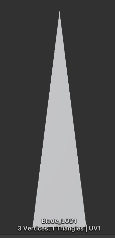
Optimization 3.1: LODs
Now that we have different chunks, we can assign specific meshes to each based on their distance from the camera. If a chunk is beyond a manually defined cutoff distance, we can load a low-level-of-detail (LOD) mesh with fewer points. Conversely, if a chunk is closer, we can load a high-LOD mesh. This approach significantly improves performance and speeds up rendering.
However, there is a visual drawback to consider. High-LOD and low-LOD meshes have distinct appearances, and as a result, a visible seam may appear when switching between LODs.

Solution Tweak 3.1.1: Fog
One solution to the problem is to make use of “fog”. Technically it’s not true fog on the grass, however, we can blend all grasses to a common color up to a distance. This doesn’t directly solve the issue from the LODs, but it does solve problems for flickering, and up to a certain point, it hides any existing seems.
Optimization 3.2: Density
Another challenge related to the grass is that, at far distances, everything tends to have a similar appearance, making it unnecessary to render a large quantity of grass blades. To address this, we can adjust the density of the grass in chunks located far away. By loading these chunks with a lower density, we can reduce the size of their compute buffers, resulting in faster culling and processing. However, a trade-off of this approach is that the grass in these far chunks may appear less dense, potentially creating a visual seam where different densities meet.
Solution Tweak 3.2.1: Increasing width
As the title suggests, one way to address the density problem is by increasing the width of the grass blades as the distance from the camera increases. By implementing a smooth transition in width from the preferred size to a final size, while simultaneously reducing the density, we can ensure that faraway chunks of grass do not appear less full compared to those closer to the camera. This technique allows for a visually seamless transition in density and width, resulting in a more consistent and visually pleasing representation of the grass at various distances.
Solution Tweak 3.2.2: Transition of density
Due to the limitations of compute buffers and to avoid the need for running the distribution shader every frame, achieving a smooth interpolation between two densities becomes more complex. In such cases, a straightforward approach is to have separate low-density and high-density chunks and load one or the other based on the distance. However, this approach introduces a seam and popping effect when transitioning between chunks with different densities.
To mitigate this issue, one option is to manually control the level of detail (LOD) for the grass objects. By setting the low-density chunk to have a quarter of the number of blades compared to the high-density chunk, we can explore two potential transition methods.
The first option is to make the grass blades that should be removed more transparent as the distance increases. However, this approach can lead to problems with transparency and clipping.
The second option is to gradually decrease the size of the grass blades until their height reaches zero. By defining a maximum distance radius around the chunk, we can ensure that once the density switches, the grass blades that are supposed to be removed have completely disappeared based on their size. This approach results in a smooth transition, involves a single value calculation during the culling process, and can be utilized as a variable in the shader for other purposes.
Optimization 3.3: Different chunk sizes
Given the low-density and high-density chunks in the scene, it is possible to optimize the representation of the low-density chunks to reduce the overall computational workload. Since the low-density chunks already process a quarter of the data compared to high-density ones, they can be made four times larger. By doing so, they will occupy more space, handle the same amount of data, and require less CPU processing.
In this optimized approach, the low-density chunks can be utilized to handle the low-density grass representation. When the camera is positioned sufficiently close to the low-density chunks, smaller high-density chunks can be loaded inside the low-density ones. On the other hand, when the camera is at a farther distance, the larger low-density chunks can be rendered. This optimization provides a performance boost as it reduces the number of distance checks, chunk loading operations, compute buffers, and dispatch calls.
While this approach has logical merits and is expected to improve performance, it may require further testing and optimization to ensure its effectiveness in practice. Nonetheless, the concept of utilizing larger low-density chunks to handle more visual data and streamline processing is a promising direction for optimization.
Applying most of the techniques mentioned in Optimization 3: Chunking
Optimization 3.4: Removing unnecessary chunks in the CPU
When using a vegetation map to distribute the grass, it is possible to encounter chunks where the distribution shader produces blades of grass with zero height. Although these blades would be removed during the occlusion culling process, we can be certain that they will never be visible. To optimize this, a simple check can be implemented during the distribution culling pass across all chunks to determine if any blades of grass are present. Since we cannot modify the sizes of the compute buffers, performing this check can speed up the CPU processing.
During the rendering process, each fragment of grass can be checked and set a boolean value indicating whether it contains grass. If no grass is present, the CPU can skip processing that particular chunk, avoiding both the draw mesh instanced operation and the occlusion culling algorithm. This optimization significantly improves performance in areas without grass, even if the viewer is observing those regions.
By efficiently skipping unnecessary computations in chunks without visible grass, this optimization technique ensures faster processing, allowing for smoother rendering in areas devoid of vegetation.
Optimization 3.5: Basic Frustum culling
Although checking at every point if it’s visible on the camera might be expensive, a simpler solution is to do a dot product of the position of the chunk with the position of the camera. If it’s negative means that is behind and never will be visible, aka, we can remove it. It’s a single line and cuts the amount of chunks to process to half of them. MORE PERFORMANCE!!
for(/*...*/)
{
    float dot = Vector3.Dot(PlayerCamera.transform.forward, section.LowLOD_Fragment.bounds.center-plannarCamera);
    if(dot < 0)
        continue;
    //...
    //Enable grass
}
Optimization 3.6: Unloading chunks
When dealing with vast world sizes, there may be instances where certain chunks remain loaded even though they are significantly distant from the camera. Although these chunks are not being processed by the CPU or utilized in any way, they still occupy compute buffers and textures, which compromises our GPU memory allocation. To address this issue, we can release all compute buffers that are not currently visible and reload them when needed. As a result, the distribution shader will be dispatched more frequently, not just once. However, this process is not significantly slow to cause any problems, and the benefit of saving space on the GPU side outweighs any potential drawbacks. The approach involves storing an object with its coordinates and associated compute buffers. By reinitializing the compute buffers while retaining the object, we can effectively manage the memory. Fortunately, the CPU has ample memory capacity, so there are no concerns on that front; it is the compute buffers that need to be cleared.

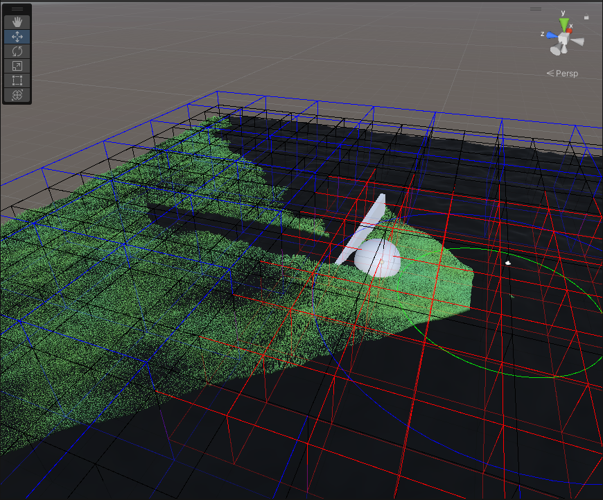
Black boxes are unloaded chunks. White boxes are loaded with chunks with no grass in them. Blue boxes are low LOD chunks with grass in them. Red boxes are high LOD chunks.
Conclusion
Following the mentioned steps produces a highly performant grass system, although there are still techniques that could be used to improve overall performance and style. There are some ideas worth checking, such as generating the mesh on the GPU and interpolating through both versions of the LODs directly.
To add up, we could add things such as a final texture to interpolate on really far grass blades, clumping different characteristics of each grass blade, or adding variety through coloring.
But for now, that’s all! Thank you for reading.