
Introduction
Since starting the grass system in my first attempt, up until now, I’ve been finding a lot of projects with similar implementations to what I’ve been looking for. Taking that into account, I’ve had to analyze, read, and understand a broad amount of different implementations to take all the benefits into account and develop my solutions.
This post will take those findings into account to explain and attempt to compare them.
Comparison
Parameters
To conduct this comparison, I have taken certain liberties to compare each of the systems. Due to the inherent differences in their methods, it is not always possible to replicate the exact same parameters, making it challenging to compare them accurately.
Therefore, please understand that there may be some approximations and rounding in order to compare the values as objectively as possible. I have made every effort to bring all systems to a similar point of comparison.
The goal is to compare each system’s rendering of approximately 2 million grass blades, considering the memory size, framerate, and flexibility to customize and modify the system according to my needs.
The systems that will be compared are:
Acerola’s Implementation
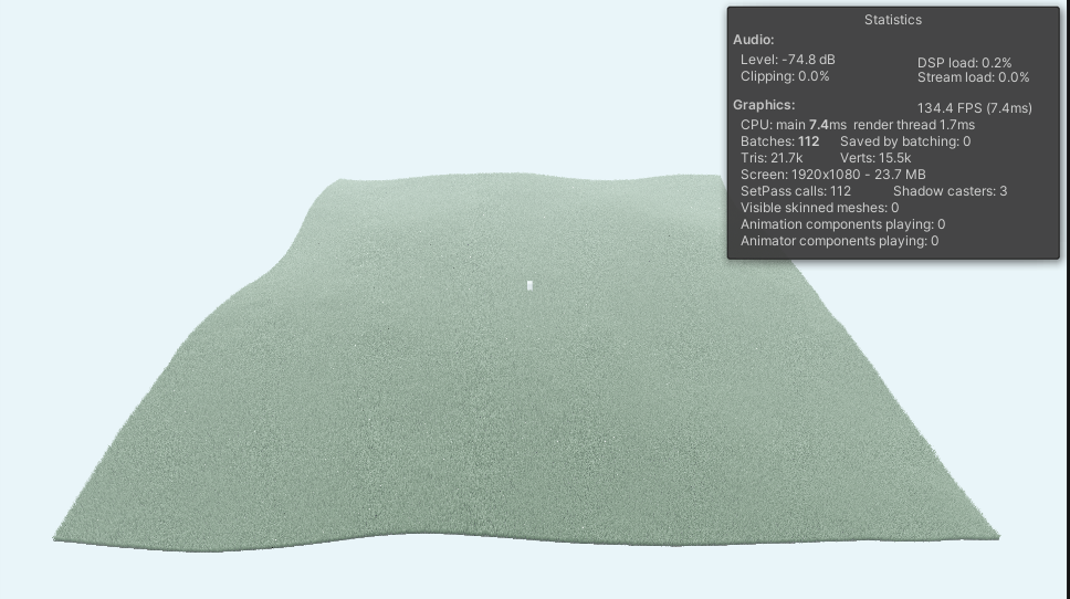
This was the initial implementation I stumbled upon, and it served as the foundation for my first solution. It’s a simple but pretty clever setup, with some clear limitations that made it a bit tricky to use directly with my procedural terrain system.
As you can tell from the pictures, the framerate and buffer size are pretty small, with 372 MB of graphics and around 140 FPS.
How it works?
This system is pretty much like my initial setup, so I won’t go into too much detail. It renders the grass in chunks, with each chunk storing the position information of every blade of grass. It utilizes an LOD (Level of Detail) system to handle rendering at various levels of detail, switching to a lower-detail mesh once a certain distance threshold is reached.
From a visual perspective, it offers some intriguing parameters. For instance, the fog effect practically erases the borders, and there are various color fields that allow for a more personalized grass appearance. On the flip side, it can be a bit challenging to get it to function smoothly with a custom or dynamic terrain because it relies on a height map texture with two height value fields. Additionally, it has limitations on the amount of grass it can render due to memory constraints, which can make it tricky to control the grass density to achieve a specific desired value. Finally, it has Frustrum Culling but not Occlusion Culling.
💡 What’s Frustrum Culling and Occlusion Culling?
Frustrum Culling is the method of discarding the rendering pass of any object that is outside of the frustrum of the camera, basically, anything that is not seen. Occlusion Culling however, is the method of discarding those elements that are behind other elements.
For each generated chunk, it starts by gathering the relevant grass positions inside it, and storing them in a compute buffer. Then, it proceeds to execute a draw call for each chunk, while implementing frustum culling in the process.
The data used for transfer is:
private struct GrassData {
	public Vector4 position;
	public Vector2 uv;
	public float displacement;
}
Which corresponds to 28 bytes per blade per data transfer.
Colin Leung Implementation
This second approach, discovered after developing my initial solution, offers a mobile-friendly solution, making it quick and cost-effective. However, it comes with the downside of limited customizable parameters.
The frame rate varies, typically hovering around 220 fps, and it keeps the graphic memory consumption quite low, at approximately 60 MB.


How it works?
In this case, we’ve got just one draw call to handle everything. We do the grass position generation on the CPU, but it’s a one-time thing during startup, and it can be quite slow. Once we’ve got all our grass blade positions sorted and stored in a single compute buffer, the system does frustum culling, and we line up a single compute shader and a single draw call for the whole grass chunk.
Customization options are kinda limited, though. Those positions have to be all lined up without any gaps to get the best performance boost from batching, so it’s not the best fit for procedurally generated terrain. The system only works with a low-res LOD blade mesh.
Plus, every grass blade keeps an eye on the camera, which makes it look nice and full, but if you peek from above, it might seem a bit weird.
The data used for transfer is:
private struct GrassData {
	public Vector3 position;
}
With a weight of only 12 bytes.
My first solution
My initial setup draws some inspiration from Acerola’s approach, with some adjustments to make it a better fit for my specific needs. It’s running at approximately 220fps and consumes around 138MB of space. However, it’s crucial to highlight that due to the system’s structure, it’s rendering considerably fewer than 2 million grass blades. Fine-tuning it to hit the mark has proven to be quite challenging.


How it works?
Instead of having each chunk render the maximum amount of grass blades, here I go for a quad-tree LOD System. This implementation can be further read at [Techniques for a Procedural Grass System] (/2023/05/Techniques-for-a-procedural-grass-system) where a clearer explanation of the different algorithms used can be found.
The transition of density has been smoothed out and therefore is not noticeable when there’s less grass in the distance. Since I made it specifically for my use case, there are all of the parameters that I would find suitable for such a system. Therefore I have full control over the looks, feel, and randomness that it requires.
The data used for transfer is:
private struct GrassData {
	public Vector3 position;
	public float displacement;
	public float cullingHeight;
}
Which corresponds to 20 bytes per blade.
My second solution
This solution, based on the implementation by Colin Leung, tries to find the best of both worlds, reducing the number of calls of different shaders but by doing so, it augments the amount of data being used. It runs at approx 300fps (the maximum available framerate on my PC) on around 337 Mb.


How it works?
Instead of each chunk storing an array with all the positions, we will only store the indices, corresponding to a singular int (instead of the previous whole GrassData struct). That alone will save a lot of memory in data transfer since only indices will be read and used for occlusion and frustum culling, speeding up the process.
However, that has an extra memory cost. The storage of all of the existing positions makes it hard to keep memory usage constrained. When the amount of chunks used increases, that value will get bigger and bigger until the point is too much for Unity to handle.
The data transfered is the same as in the first solution and therefore it uses 20 bytes per blade. The parameters used are the same as in the first solution proposed.
Direct Comparison
| 1st | 2nd | 3rd | 4th | |
|---|---|---|---|---|
| Framerate | Second Solution (297 fps) | First Solution (220 fps) | Colin Leug (220 fps) | Acerola (140 fps) |
| Memory Used | Colin Leug (60 MB) | First Solution (138 MB) | Second Solution (237 MB) | Acerola (372 MB) |
| Customization | Second Solution = First Solution | Acerola | Colin Leug |
Another Factor enters the game!
One thing that I barely talked about yet is scalability. Each system has its glory somewhere. However, how well does each method scale?
Coling Leung implementation stays at a consistent framerate with more and more blades, keeping it pretty consistent.
The first solution will not increase too much in memory with bigger chunks, but the framerate will take a big hit the more amount of blades to render. The second solution has the opposite problem. The framerate will stay consistent, but the memory budget will be quickly killed.
That makes neither of the two the best approach. In an infinite procedural world (and in all cases), you want to keep the memory low, while keeping the framerate high. Although the memory cost and framerate will vary, the more consistent the system is, and the less it varies with more requests or variations, the better the system will be. If I wanted to add trees, more grass blades, bushes, rocks, or other props using the same system, it would, in both cases, perform poorly. So what could I do? Ideally, Coling Leung implementation would be great, since it’s extremely quick with a really low budget. However, the lack of customization would be a problem for a procedural terrain, where I would be interested in making regions without grass or the use of different meshes.
A third solution?
Taking all of this into account we can see that there’s clear room for improvement, a third solution. A system that allows both, high framerate and low memory cost. If we could do a system that doesn’t cost us more memory the more data needs to be processed, we would also save framerate. Indirectly, having less data on the GPU will give us more room for other effects later on.
The final system (Finally this is working as I would like)
Coming from the second solution we can see what’s the clear drawback, the high memory cost. That’s because at the start of the game, the system generates all of the grass positions in a singular mesh, making it dependent on the size of the mesh, and therefore it will scale poorly. If the size of the mesh is too big, the request for grass positions is going to kill the budget of the GPU and CPU.
In contrast, the use of indices to quickly select the data that we will use is the quickest and the cheapest of the options. So what can we do to get the final solution?
Don’t store the positions!
I’ve kept generating the positions in all attempts because I thought that that process would be slow and expensive. If I avoided doing that at every frame I would save time and resources. But I didn’t check if that was true or not. What was going to happen if I didn’t store it, and instead, generated it at every frame? Well, the results were impressive.
The idea is at generation, we schedule and create each of the chunks that will have grass data, and that will be used for culling. That doesn’t require the positions yet, so no problem there.
Now we get the indices of that chunk that will require a grass blade, but oh, I need the positions to know what needs to be put here! Well, don’t worry!
I will just calculate them, get the grass position according to the index, and store it if it’s valid or not. We are not going to store all indices, just the ones that exist. Furthermore, in this step, we can do a check to know if there’s even a blade in the chunk or not, and if there isn’t, we will just throw away the whole chunk, marking it as empty, so no calculations will ever be run again there.
[numthreads(8,8,1)]
void SelectIndices(uint3 id: SV_DISPATCHTHREADID){
	if(id.x < _InstancesInChunk && id.y < _InstancesInChunk){
		int2 xy = id.xy*indexMultiplier+int2(IndexOffsetX, IndexOffsetY);
		int index = xy.x+xy.y*_TotalInstances;
		GrassData data = GetGrassDataFromIndex(index);
		if(data.height > 0){
			_Indices.Append(index);
		}
	}
}

GrassData GetGrassDataFromIndex(int index){
	float2 fractalIndex = GetFractalIndex(index);
	GrassData finalData;
	if(fractalIndex.x <= 1 && fractalIndex.x >= 0 && fractalIndex.y <= 1 && fractalIndex.y >= 0){
		finalData = CalculateInterpolatedGrassData(fractalIndex, index);
	}
	else{
		finalData.position = 0;
		finalData.height = -1;
	}
	return finalData;
}
Now we’ve done the initial part, all the data needed is prepared and ready for the rendering pass. We will store those valid indices, into a compute buffer in each chunk.
Let’s move to the rendering part!
The process will make us go through each available chunk. First, we get the indices and the dispatch arguments, that are in the different compute buffers and we will start running the required compute shaders. In each chunk, we will recalculate the positions, perform occlusion and frustum culling, and set that final information into a single compute buffer. At the same time, we will fill two separate compute buffers with the indices related to a HighLOD, and a LowLOD.
With that, we will do a render call for both LODs, using the required dispatch arguments (those that define how many blades to render).
for(int i = 0; i < LowLODBlade.ArgumentsBuffer.Length; i++){
	//This is a setup to be able to work with submeshes for more complex meshes
	ComputeBuffer buffer = LowLODBlade.ArgumentsBuffer[i];
	commandBuffer.CopyCounterValue(LowLODIndices, buffer, sizeof(uint));
	commandBuffer.DrawMeshInstancedIndirect(LowLODBlade.bladeMesh, i, LowLODBlade.materials[i],
		passIndex, buffer, 0,propertyBlock);
}
As you can see in the previous code, we are making use of a Command Buffer. This allows us to schedule the call to a defined step in the frame call, but also, so that not all the dispatch calls happen instantly. Normally a DrawMeshInstanced will be scheduled with the defined Compute Buffers to a later point in the update method, while the dispatch calls will generally be scheduled as soon as possible.
That would make it so that this system wouldn’t work. At each dispatch call, the compute buffers would get the data overridden (like the positions), and once it gets to the time to render, the data to render will be random and the same for each render call.
Instead, by using the Command Buffer, we can make sure that each render call will only be executed right after all the dispatch calls, and before running the next chunk.
In conclusion, that means that the memory cost, since we are reusing the same compute buffer for all the chunks, will be, in worst case scenario, the max size of our chunk of grass, and it will not scale with draw distance, visibility, mesh scale, etc… This makes it slightly slower but with an extremely low memory cost.
Final comparison
Well sadly, at the making of this blog, the whole project has already evolved, including many other subparts that don’t allow for such a straightforward screen capture.

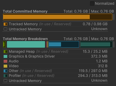
Here we can see the closest that resembles information regarding the whole system. In this case, around 37.1 MB is reserved for only the rendering, which includes the compute buffers used and the different graphics buffers to be able to render the system.

Regarding performance, in this picture, we can see that the performance runs around 130 fps.
However, both the performance and the memory cost of this new system are not truly represented in these pictures. As said at the beginning of this chapter, other things are going on in the background that collude with the grass system, making it so that this doesn’t truly define the improvements.
The memory cost remains low, even when making the chunks hugely bigger, and does not increase almost at all when adding other elements (such as trees, rocks, or other props). The performance now stays constrained by the CPU speed of processing each of the elements, giving us room to improve it even more in the future.
Conclusions
The hardest part of this blog has been the comparison of the different systems itself. It’s quite hard to get similar settings on systems that are built completely differently and even harder when hidden settings are making some setups harder than others. It is for that that I wouldn’t recommend taking these results at face value since they might greatly change between systems or even sessions.
The general idea, however, should stay the same.
Thanks to the low cost of this solution, I managed to implement, using the same system, rendering of other meshes. With a couple of changes to the settings of the grass, some generalizations on the grass shader, and tweaks here and there, we can render trees, bushes, rocks, and other elements.
In addition, if we get the positions of the vegetation, after calculating it for the first time, we can spawn the required colliders for trees or big rocks, making it tweakable.
Some changes and extra settings can be added. First of all, allowing multiple LODs, rather than only two would greatly improve performance and customization for deciding the look of any vegetation. In addition, we could add rotation, custom collision meshes, a scale factor, or more settings per grass structure (Now that the memory cost is so little) so we have more control over the final look of the vegetation.
If that increases too much, maybe it’s interesting to split it back into two structs, one for the grass, and one for the rest of the vegetation, although I’m still not sure about it.
To sum up, this solution seems to be performing great with little memory cost, it works in real-time and it’s better than any of the previously analyzed solutions.